Autonomous Drilling Console
- Apr 6
- 20 min read
Updated: May 13
Magna-1-Z Well | Adaptive Steering Intelligence ·| ML Level 1 | Python · Plotly Dash · NumPy
"15 Years of Well Planning + Directional Drilling Experience — Encoded in Software"
1. About This Project
The Autonomous Drilling Console is a full-stack, real-time directional drilling simulation built entirely from first principles. It was developed to demonstrate how 15 years of hands-on well planning and directional drilling expertise — from designing 3D well trajectories to reach geological targets, to steering a wellbore through thousands of metres of rock in real time — can be translated into working, intelligent software.
The console autonomously drills a deviated wellbore on the synthetic Magna-1-Z well — a purpose-built simulation well with realistic trajectory data, designed to represent a typical deviated wellbore scenario without using any real client or operator data. It generates synthetic Measurement While Drilling (MWD) survey stations every 28.5 metres using the Minimum Curvature Method (MCM) — the industry-standard algorithm for computing 3D wellbore position from inclination and azimuth readings. It continuously computes Travelling Cylinder Plot (TCP) geometry to measure the precise 3D offset between the actual well position and the planned well trajectory. Based on this, it calculates the correct Toolface angle and Rotary Steerable System (RSS) Deflection percentage to steer the well back to plan — accounting for the formation's natural right walk tendency, the Dogleg Severity (DLS) variation with inclination, and the 3D coupling between build rate and walk rate.
The system learns from each stand it drills. Using an adaptive machine learning algorithm, it updates its estimate of tool effectiveness (EM) and right walk rate (RW) from observed versus predicted build and walk rates after every 28.5 metre stand. Each successive recommendation becomes more accurately calibrated to real formation behaviour — exactly as modern autonomous drilling advisory systems operate in the field.
This project was built through 20+ development iterations across two major versions, systematically testing physics formulas, discovering real errors in sign conventions and coupling assumptions, and fixing each one through careful analysis of drilling behaviour. Every bug found and fixed was a real directional drilling insight — not just a software error in the conventional sense.
"What does directional drilling mean for someone not from the oil and gas industry?"
Directional drilling is the process of steering a wellbore through rock at depths of hundreds or thousands of metres — underground, with no GPS, no line of sight, and measurements taken only every 28.5 metres. The driller must decide — at each measurement point — what angle and power setting to command to a downhole motor, knowing that the formation itself resists and deflects the tool unpredictably. This console automates that decision-making process using physics-based algorithms and machine learning, achieving 88.9% autonomous control over 510 metres of simulated drilling with only 2 human interventions.
2. Project at a Glance
Stands drilled (demo) | Depth drilled (demo) | Distance — auto mode | Distance — manual mode | Total commands | Auto commands | Manual commands |
20 | 541.5 m | 502.4 m / 93% | 39.1 m / 7% | 57 | 54 / 95% | 3 / 5% |
Note: The statistics above reflect a complete demo run of 541.5 metres (20 full stands) on the synthetic Magna-1-Z well, drilled from 880.85m to 1422.35m measured depth. This is a more thorough run than the initial demo — twice the depth, three times the command volume, and demonstrably stronger ML Level 1 learning evidence. Results will always vary depending on user manual input choices — the system adapts its recommendations to each decision made in real time.
3 Live Console — Try It Now
Drilling is a game of patience — and so is this demo. Treat it as real drilling, take your time, and put the autonomous intelligence to the test. Each stand takes roughly 2-3 minutes. Accept the auto-commands, observe the well trajectory build, and watch the system self-calibrate. The deeper you drill, the smarter it gets.
No installation required · Opens in browser · Press ▶ to begin · Allow 30-40 minutes for a full 10-stand run
🔗 Click to open the Live Console in separate browser
4. Autonomous Drilling Performance — 500m Demo Run
Demo Result Summary
The system completed 20 full stands of drilling on the synthetic Magna-1-Z well — from 880.85m to 1422.35m measured depth, a total of 541.5 metres. Only 3 manual commands were given in 57 total downlink interactions (5%), covering just 39.1m (7%) of total distance. The remaining 502.4m (93%) was drilled entirely under autonomous control. The system demonstrated clear Machine Learning Level 1 formation calibration — progressively adjusting deflection from 50% at stand 1 to 75-80% by stands 11-12 as it learned the formation was under-delivering theoretical build rate, then intelligently reducing back as the well converged with the plan.
The system autonomously reversed its steering strategy at two plan-crossing events with no human input at either crossing.
Key Autonomous Decisions
(★ = mid-stand auto correction · ★★ = major autonomous strategy change · ML = ML Level 1 learning visible)
The following table captures the most significant autonomous command decisions — moments where the system changed toolface or deflection based on formation feedback, ML calibration, or TCP geometry. Only major decisions are shown; the full 57-command log is in the detail table below.
MD (m) | Stand # | New TF / Defl | Previous TF / Defl | System Reasoning |
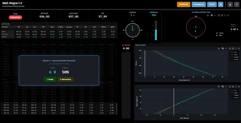
890.45 | 1 | 3 L / 50% | — / — | First stand. Survey 2.48m from plan. System initiated 3° Left toolface from the very first command — recognising the formation's natural right walk tendency (RW=0.271°/30m) and pre-compensating. This was not reactive; the system computed the correct direction from TCP geometry before any drilling had occurred. |
965.35 ★★ | 4 | 3 R / 50% | 0 HS / 50% | Major toolface switch: 0 HS → 3R. Plan azimuth is now pulling rightward ahead of the survey. System detected crossing_imminent (plan azimuth within 1° when projected 1 stand ahead) and entered Phase B — begin converging rightward toward plan azimuth. Maintains 50% deflection while introducing rightward walk. The plan comes to us; we begin converging. |
1050.85 ★★ | 7 | 0 HS / 55% | 3 R / 55% | Switch from 3R back to 0 HS. Azimuth on plan. System re-enters Phase A — hold azimuth while continuing to build. Slight deflection increase from 50→55% suggesting ML Level 1 is beginning to note that formation delivers slightly less build rate than theoretical. Clean Phase B→C→A transition visible here. |
1079.35 ★★ ML | 8 | 0 HS / 40% | 0 HS / 55% | Deflection dropped sharply 55→40%. Survey Inc variance is now positive (survey above plan in TVD). System correctly detected it is building faster than plan requires and needs to slow down aggressively. The 15% deflection reduction shows confident, bold autonomous action — not a gradual step. Without this, the well would have over-shot the plan line from below and required expensive correction. |
1156.55 ★ ML | 10 | 0 HS / 45% | 0 HS / 40% | Mid-stand. Deflection increased 40→45%. Well has touched the plan line but ML Level 1 is now adjusting — the formation is under-delivering build rate compared to prediction. System increasing power to maintain position on plan rather than falling below it. First sign of the upward ML calibration trajectory that will continue through stands 10-12. |
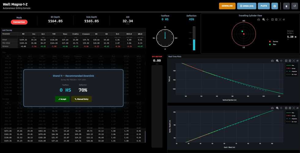
1164.85 ★★ ML | 11 | 0 HS / 70% | 0 HS / 40% | Most dramatic single deflection jump in the run. 40→70% in one command. Survey has fallen below plan — TCP 1.28m. ML Level 1 has now calibrated that this formation requires significantly more power than theoretical. After stands of conservative 40-45%, the system understood the formation is soft and responded with a bold 75% correction. This is formation learning at its most visible — the system changed its model of the rock and acted accordingly. |
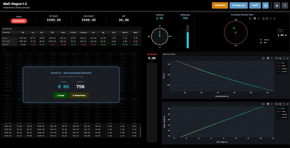
1193.35 ★★ ML | 12 | 0 HS / 75% | 0 HS / 70% | Further increase 70→75%. Survey still below plan (TCP 1.99m). System has not yet caught up and continues to increase power incrementally. The ML-calibrated EM estimate is driving higher deflection than the uncalibrated baseline would ever have commanded. Without ML Level 1, the system would have stayed at 50% and never caught the plan in this formation. |
1213.55 ★★ | 12 | 3 L / 75% | 0 HS / 75% | Toolface switch HS→3L while maintaining 75% deflection. Survey has drifted azimuth-right of plan — TCP shows lateral (rs) component. System enters Phase C correction for azimuth while simultaneously maintaining maximum vertical build power. This is a true 3D simultaneous correction — toolface adjusted for azimuth while deflection holds for TVD recovery. The simultaneous 3D solver is doing exactly what it was designed for. |
1335.85 ★★ | 17 | 0 HS / 60% | 3 L / 65% | Toolface back to 0 HS, deflection reduced 65→60%. Azimuth correction complete — survey back on plan azimuth. Deflection reduction signals system is satisfied with vertical position and beginning to ease toward maintenance mode. TCP distance 1.30m — within acceptable range. A planned, controlled de-escalation of correction intensity. |
The progressive deflection journey across this demo — 50% → 75% → 50% — is the most complete demonstration of ML Level 1 formation learning to date. The system started at theoretical baseline, learned the formation required more power, corrected aggressively, caught the plan, then de-escalated as conditions stabilised. All autonomous. All without being told a single fact about the formation.
Full Command Detail Log
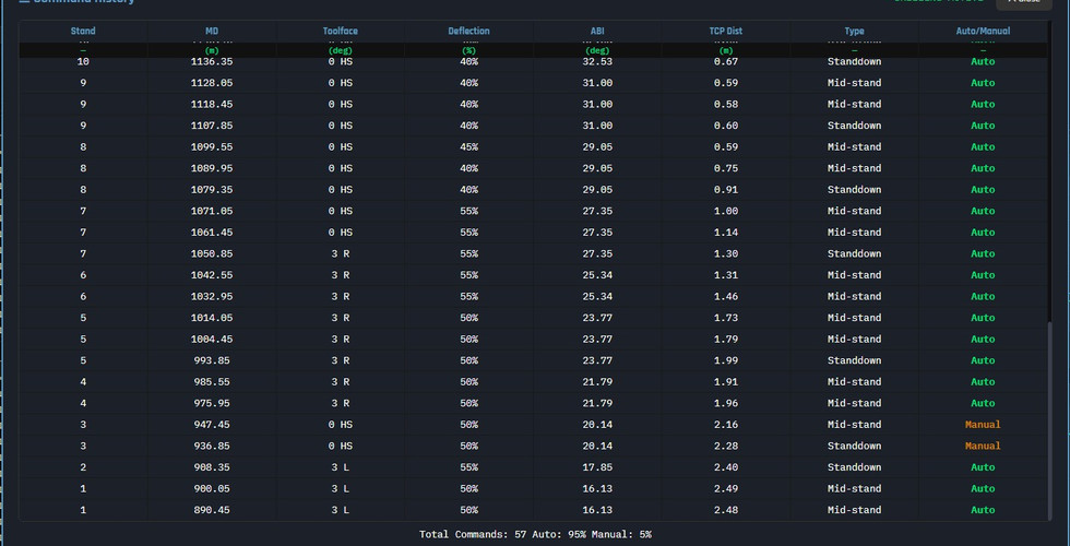
A complete 57-command log with individual observations for every auto and manual command is provided in the downloadable Excel file below. It documents the reasoning behind each toolface and deflection decision across all 20 stands — including the incremental ML Level 1 calibration progression visible through the deflection trend from stand 1 (50%) to stand 12 (75%) and back to stand 20 (50%).


(Click Next to view slideshow)
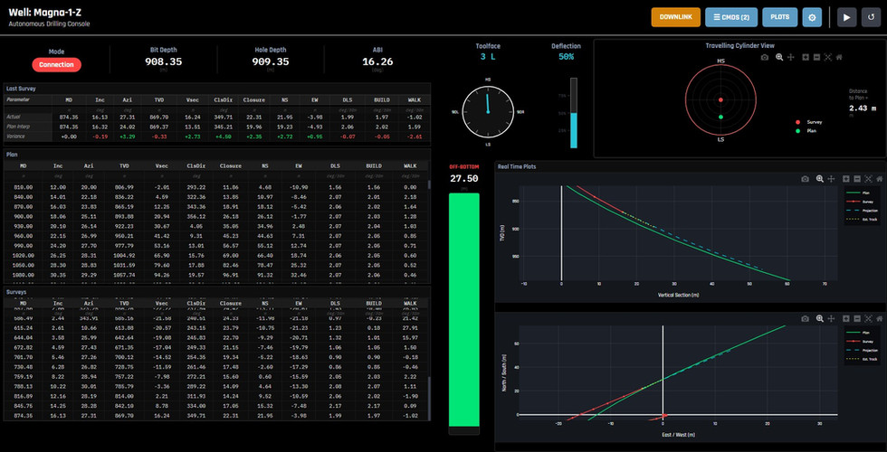
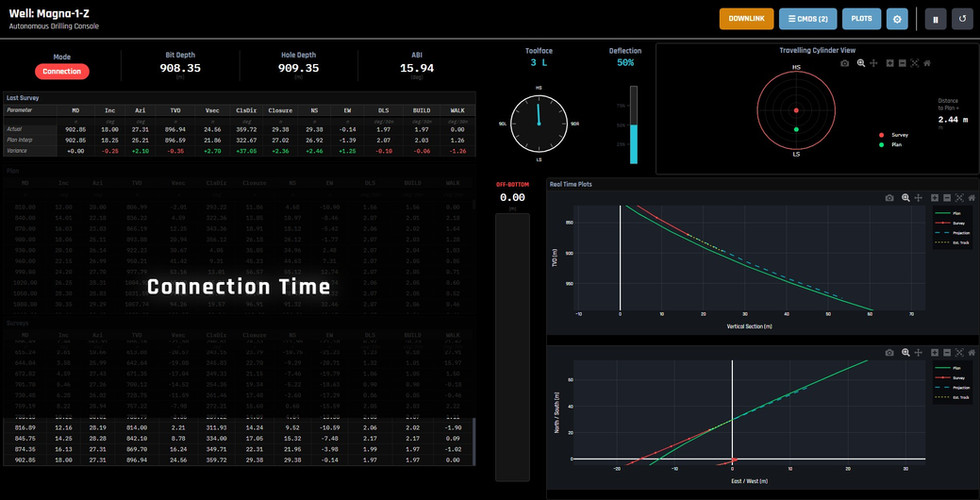
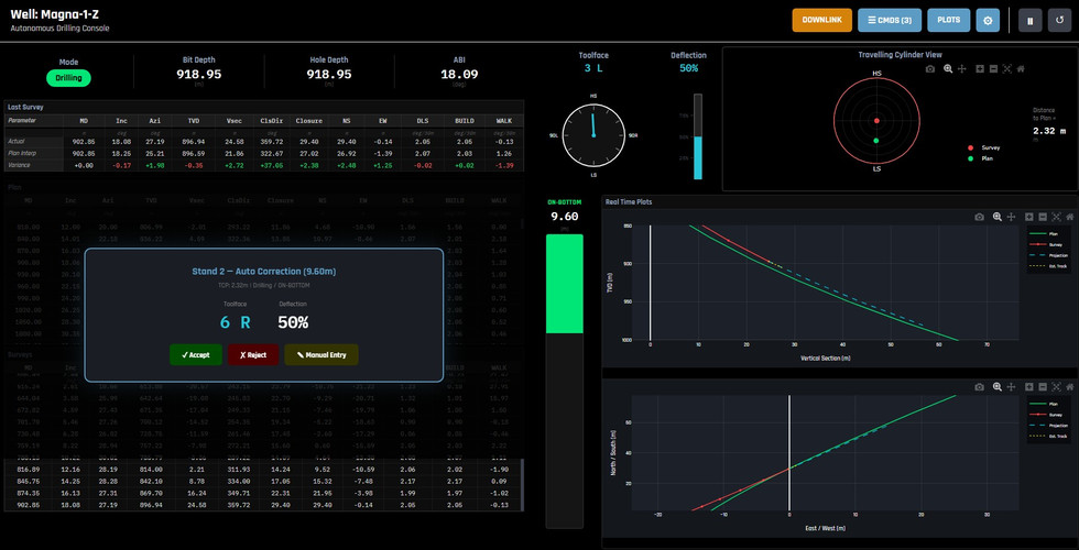
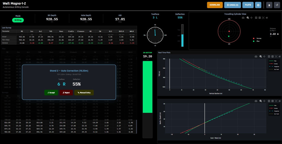
Screenshot Gallery
A slideshow of all screenshots from this 541.5m, 20-stand demo run is included below. These images show the well trajectory at each significant stand, the TCP dial readings, the auto-generated downlink popups, and the full command history panel. Note that your own run will produce different trajectories and recommendations depending on your manual input choices — the system adapts to each decision in real time.


(Click Next to view slideshow)


(Click Next to view slideshow)
5. How to Use the Console
Quick Start — 3 Steps
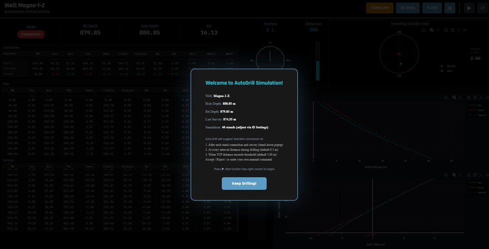
Click the Live Console link in Section 3 above → page loads with the Welcome screen
Click "Keep Drilling!" to dismiss the welcome popup
Press the ▶ Play button (top-right corner) → drilling starts autonomously
The system will drill stand by stand, generating downlink recommendations at each stand-down and mid-stand interval. You can accept, reject, or manually override every recommendation. The well trajectory updates live in the Real-Time Plots section.
Header Buttons — Control Panel
Control | Location | What it does |
▶ Play | Top-right header | Starts the drilling simulation from kick-off depth. Well begins drilling automatically. |
⏸ Pause | Top-right header | Pauses drilling at any point. Can be resumed at any time. |
↺ Reset | Top-right header | Resets entire simulation back to Stand 1 at original depth. |
DOWNLINK | Top-right header | Opens manual downlink panel to send a custom toolface and deflection command at any time. |
☰ CMDS (N) | Top-right header | Opens full command history — every auto and manual command logged with stand, MD, TF, Defl, ABI, TCP distance and Auto/Manual flag. |
PLOTS | Top-right header | Opens full-screen well trajectory viewer with zoom — Vertical Section and Plan View with all traces. |
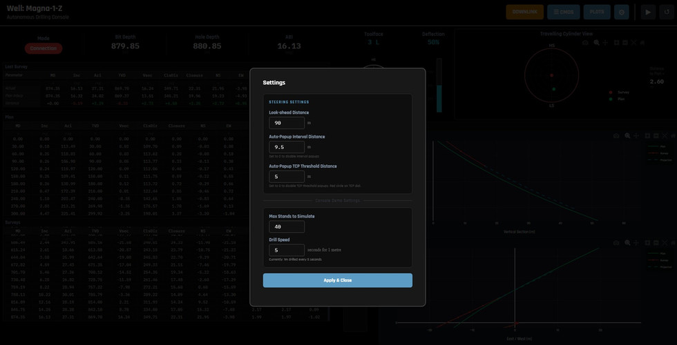
⚙ Settings | Top-right header | Configure lookahead distance, max stands, auto-popup interval, TCP threshold, and drill speed. |
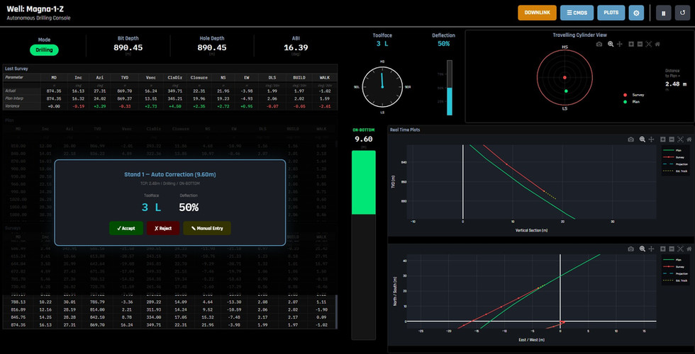
✓ Accept | Popup dialog | Accepts the system auto-generated toolface and deflection recommendation for this stand or mid-stand correction. |
✗ Reject | Popup dialog | Rejects recommendation and continues drilling with previous active toolface and deflection settings. |
✎ Manual Entry | Popup dialog | Opens input fields to enter your own toolface (0–177° L/R/HS/LS) and deflection (%) values. |
⚙ Settings Panel — Configurable Parameters
Setting | Range / Default | Effect |
Look-ahead Distance | 30–300 m (default 90 m) | Controls how far ahead the projection arc is calculated. Shorter = more reactive. Longer = more predictive. |
Max Stands to Simulate | 1–40 (default 15) | Total number of stands before the simulation ends automatically. |
Auto-Popup Interval | 0 = disabled (default 9.5 m) | System automatically pauses mid-stand and generates a correction popup every N metres drilled within a stand. |
Auto-Popup TCP Threshold | 0 = disabled (default 5.0 m) | System generates a correction popup when the well deviates this far from plan in TCP distance. |
Drill Speed (sec/m) | Min 1 (default 5.0) | Controls simulation speed. Lower value = faster drilling. Set to 1 for rapid testing. |
Understanding the Live Display
TCP Travelling Cylinder View (top-right): Red dot = current survey position. Green dot = where the plan line is. Distance in metres = your steering error in 3D space.
Toolface Dial: Orange compass needle. Straight up = 0° toolface (High Side, pure build). Clockwise = Right toolface. Anti-clockwise = Left toolface.
Deflection Bar: Vertical orange bar. Higher bar = more aggressive build/walk rate. 100% = maximum tool capability.
Vertical Section Plot: TVD vs Vsec. Green = planned well. Red = actual surveys. Cyan dashed = projection arc. White dashed = estimated bit position.
Plan View Plot: North/South vs East/West — bird's eye view showing azimuth behaviour.
Last Survey Table: Three rows — Actual, Plan interpolated at same depth, and Variance. Green = ahead of plan, Red = behind plan.
⚠ Important — Your Results Will Differ
The demonstration screenshots show results from one specific test run where mostly auto-commands were accepted. If you use Manual Entry to override the auto-generated recommendations, the well trajectory will follow your choices from that point onward, and subsequent auto-commands will be recalculated based on the new well position. The end results are completely dependent on the combination of auto and manual choices made during each run. This variability is intentional — it demonstrates that the system responds and adapts to real-time human decisions.
6. Well Planning & Directional Drilling Knowledge — Encoded in Software
My career has spanned well planning and real-time directional drilling across multiple basins and well types — from designing 3D well trajectories to reach geological targets, to steering in real time using Measurement While Drilling (MWD) data from downhole tools. This combination of pre-well planning (where the well should go) and real-time execution (how to steer it there) is rare in a single practitioner. Every concept below was implemented from direct field experience.
➡ Minimum Curvature Method (MCM) — Industry Standard Wellbore Position Calculation
MCM is the universally accepted algorithm for computing 3D wellbore position (True Vertical Depth, North, East) from survey stations (Measured Depth, Inclination, Azimuth)
Ratio Factor RF = (2/DL) × tan(DL/2) — correctly degenerates to RF=1.0 for straight sections when Dogleg angle DL < 1×10⁻¹⁰
Every synthetic survey station in the simulation is generated using MCM from the previous station plus commanded toolface and deflection
All TVD, NS, EW, Vsec and closure values validated against the real Magna-1-Z plan data interpolated from the well CSV file
➡ Dogleg Severity (DLS) Variation with Inclination — Non-Linear Walk Rate
Dogleg Severity (DLS) = angular change per 30m of drilling — the key measure of wellbore curvature. The same toolface and deflection produces different walk rates at different inclinations
Walk rate formula: da/stand = (adls × sin(TF) / sin(Inc) + RW) × (CL/30) — the sin(Inc) denominator is the critical coupling term
At Inc=20°, sin(Inc)=0.34 → toolface contribution is amplified ~3× → small TF changes cause large azimuth effect. At Inc=60°, sin(Inc)=0.87 → far more stable and predictable
Dynamic toolface cap implemented: ±45° when walk ≤ 1°/30m (build-dominant), ±177° when walk > 1°/30m (turn-dominant)
All formulas tested across the full inclination range of this well (0° to 50°+) and results validated against plan DLS column at each depth
➡ Right Walk Tendency (RW) — Formation Constant That Must Always Be Cancelled
Real Rotary Steerable System (RSS) tools have a natural right walk tendency — they drift rightward regardless of commanded toolface
RW = 0.271°/30m for the Magna-1-Z formation — this value is always present and must be accounted for in every toolface calculation
Without RW cancellation: commanding "hold azimuth" (toolface = 0) actually drifts right by 0.27°/30m — nearly 0.81° per 3 stands
Correct toolface inversion: sin(TF) = (target_walk − RW) × sin(Inc) / adls — RW subtracted from target walk before solving for TF
Applied in EVERY toolface calculation: popup recommendations, projection arc, mid-stand corrections, and ML Level 1 RW estimation
➡ Catching Plan with a Smooth Corrective Arc — Gradual Convergence
Field principle: never make abrupt corrections — approach the plan line in a smooth, controlled arc to avoid overshoot
Survey above plan → reduce deflection to 35–40% → build rate slows → well curves gently back toward plan from above
Survey below plan → increase deflection to 60–65% → accelerated build rate → catches plan in a smooth arc from below
Variable lookahead: system searches 28.5m to 150m in one-stand steps to find the optimal distance where required DLS to reach the plan equals plan DLS at that depth (±0.5°/30m tolerance)
The projection arc endpoint always connects to a physically meaningful point on the plan line — not at an arbitrary fixed distance
➡ 3-Phase Azimuth Strategy — Phase A (Hold) / Phase B (Converge) / Phase C (On Plan)
Phase A — HOLD: Survey is ahead of plan in azimuth. Command 6° Left toolface to cancel RW and hold azimuth steady. Let the plan line (turning right) catch up naturally. Do NOT prematurely turn right.
Phase B — CONVERGE: When plan azimuth projected 1 stand (28.5m) ahead is within 1° of survey azimuth → begin gentle rightward turn (plan_rate + 0.1 to 0.3°/30m extra)
Phase C — ON PLAN: Match plan turn rate exactly with graduated corrections of 10°→20°→30°→45° based on TCP lateral distance (rs component)
Key insight: Phase B trigger compares plan azimuth at MD+28.5m versus current survey azimuth — the PLAN comes to US, not us chasing the plan
➡ Simultaneous 3D Vector Solver — TF and Deflection Are Coupled in 3D Space
Moving toolface away from High Side (HS) reduces the build component by cos(TF) AND increases the walk component by sin(TF) simultaneously
These two effects cannot be optimised independently — they require a single combined 3D vector calculation
Correct solution: walk_comp = (target_walk − RW) × sin(Inc)
TF = atan2(walk_comp, target_build) → Defl = sqrt(target_build² + walk_comp²) / FMXB × 100
This achieves BOTH the target build rate AND the target walk rate simultaneously in one combined calculation
➡ Travelling Cylinder Plot (TCP) — Geometry, Sign Conventions and Steering Trigger
TCP projects the planned well trajectory onto a plane perpendicular to the actual wellbore direction at the current survey station
hs component: High Side / Low Side offset — hs negative means plan is below the survey in the HS direction
rs component: Right / Left offset — rs positive means plan is to the RIGHT of the survey → must turn RIGHT to correct
Critical sign fix discovered in testing: hs = −dot(d2, HS) must be negated. Without this, HS and LS directions are completely swapped
TCP calculation vectorised using NumPy dot products — approximately 0.04ms per call, continuously updated during drilling every 2 metres
➡ BHA Response Modelling — Formation Noise and Tool Effectiveness
BHA (Bottom Hole Assembly) response is never exactly as commanded — formation variability, bit-rock interaction and tool wear all cause deviation
Tool effectiveness EM modelled as Normal distribution (mean=1.0, standard deviation=0.08) — each stand delivers a slightly different fraction of theoretical capability
Formation noise MN=0.3° applied independently to inclination and azimuth with correlated amplitude clipping — realistic survey-to-survey variability
Build rate schedule varies by stand number (2.2 → 1.6 → 2.6°/30m) matching the actual planned well program
Random seeds fixed at seed=42 for reproducibility — same inputs always produce the same base synthetic trajectory
7. Technical Skills
Skill Area | Description |
Well Planning & Directional Drilling Concepts | Minimum Curvature Method (MCM), Dogleg Severity (DLS) calculation at varying inclinations, Travelling Cylinder Plot (TCP) geometry and sign conventions, right walk tendency (RW) modelling, 3-phase azimuth strategy (Hold / Converge / On Plan), smooth corrective arc planning, toolface and deflection 3D coupling |
Python Application Development | Full-stack Dash application (2,375+ lines single-file), dcc.Store state management, dual-timer architecture (iv-fast + iv-phase), race condition prevention, multi-output Dash callbacks, Plotly figure optimisation (2m boundary rendering to prevent browser lag) |
NumPy and Pandas Data Engineering | Vectorised Travelling Cylinder Plot (TCP) calculation using NumPy dot products (~0.04ms per call), pre-computed plan point arrays, Pandas CSV interpolation for plan and survey data, exponential moving average (EMA) for ML Level 1 updates |
Machine Learning — Adaptive Formation Learning (ML Level 1) | Exponential Moving Average (EMA) based EM (tool effectiveness) and RW (right walk rate) calibration per stand. Update conditions: EM when cos(TF) > 0.15 (build component reliable); RW when abs(TF) ≤ 9° (walk dominated by RW). Convergence within 5–6 stands. Mirrors formation characterisation approaches used in commercial autonomous drilling advisory systems. |
3D Simultaneous Steering Solver | Vector decomposition: TF = atan2(walk_component, build_component); Defl = sqrt(build² + walk²) / FMXB × 100. Dynamic toolface cap ±45° (build dominant) / ±177° (walk dominant). Deflection 100% cap with toolface recovery logic to maximise build rate. |
Software Architecture & Iterative Design | Phase state machine (12 phases: welcome → run_to_bottom → drilling → standdown_pause → connection time → survey time → survey display → popup → downlink sequence → done), 20+ iteration bug-fix cycle, performance optimisation (0.3ms dynamic projection search), command history logging with Auto/Manual tracking and live percentage statistics |
8. Development Journey — 20+ Iterations
Built through systematic iterative development. Each iteration addressed a specific physics hypothesis, operational concept, or system behaviour — tested by running the simulation and observing results against expected drilling outcomes:
Version | Key Developments |
v1 — Foundation | MWD survey monitoring, plan vs actual comparison, Vsec and Plan view trajectory plots, TCP dial, static downlink popup workflow |
v2 itr1–2 — Popup Workflow | Hidden placeholder fix for all callback IDs, pp_reject re-enables iv-fast (prevents frozen drilling), Stand 1 depth reset fix, complete reset button restoring all 23 display elements |
v2 itr3–4 — Projection Redesign | clean_gen_survey() deterministic corrective arc (zero noise), projection stored in Store once per stand, proper MCM physics in survey generation, TCP-based auto_cmd rewrite |
v2 itr5 — TCP Sign Fix | Critical: hs = −dot(d2, HS) must be negated. Without this HS/LS directions completely swapped — all vertical corrections went the wrong way |
v2 itr6–7 — TCP Steering + RW Cancellation | tcpsteer() simultaneous 3D solver, RW-aware 3-phase azimuth A/B/C, Phase B detection (plan comes to us), dynamic TF cap 45°/177°, auto browser launch |
v2 itr8–9 — Projection Geometry | Phase 3 forward-MD interpolation, EW/NS position matching, MIN_STEPS=4 fix (Stand 1 missing projection), max_iter=20 infinite loop guard, counter-correction sign fix in 0.5–1m zone |
v2 itr11 — Dynamic Lookahead | 28.5–150m adaptive lookahead search (6 iterations, ~0.3ms), DLS tolerance ±0.5°/30m, projection endpoint guided to plan line, default 90m lookahead, max 15 stands |
v3 itr1 — ML Level 1 + CMDS Panel | Adaptive EM and RW estimation (EMA α=0.3), fmt_tf() full 0–177° range support, ☰ CMDS command history panel with live Auto/Manual tracking and badge count |
v3 itr2 — Steering Logic Fix | rs sign corrected in Phase C (rs>0 → turn RIGHT, was incorrectly LEFT), plan_rate contamination removed from catch-up branch, ML estimates wired through all projection and auto_cmd calculations |
9. ML Level 1 — Adaptive Formation Learning
After every stand-down, the system compares what was commanded versus what the wellbore actually delivered, and updates its internal formation model:
How it works — per stand (every 28.5m)
Observe actual build rate and walk rate from new MWD survey
Compare with predicted build and walk from commanded TF and Defl
Update EM_estimated (tool effectiveness) from build error
Update RW_estimated (right walk rate) from walk error
All subsequent recommendations use calibrated estimates
Converges to true formation values within 5–6 stands
Mathematics — α = 0.3 learning rate
EM_est = EM_est × 0.7 + correction × 0.3
When cos(TF) > 0.15 — build component is reliable
RW_est = RW_est × 0.7 + obs_walk × 0.3
When abs(TF) ≤ 9° — walk dominated by RW not sin(TF)
Evidence in the 541.5m Demo Run — 20 Stands
Deflection signature — the complete learning cycle: System started at EM=1.0 theoretical (50% deflection at stand 1). By stands 8-9 it correctly reduced to 40% detecting over-build. By stand 11 it jumped to 70%, stand 12 to 75% — having learned the formation under-delivers build rate. By stand 14 it was de-escalating back to 65%, stand 17 to 60%, and by the final stand 20 it returned to 50%. The full arc — 50% → 40% → 75% → 50% — across 20 stands is the most complete ML Level 1 calibration cycle demonstrated on this well.
Toolface evolution — 4 distinct phases: 3L (stands 1-2, azimuth correction) → 0 HS (stand 3, azimuth on track, pure build) → 3R (stands 4-6, Phase B converge toward plan azimuth) → 0 HS (stands 7-14, on plan, pure build with ML-calibrated deflection) → 3L (stands 12 mid, 15-20, azimuth drift correction and plan turn). Each transition was autonomous, driven by TCP geometry and RW_estimated updates — no human guidance on toolface across 17 of 20 stands.
Formation softness discovery at stand 11: The single most revealing ML moment — after stands of 40-45% delivering insufficient build rate, the system jumped to 70% deflection in one command at MD 1164.85m. This 25% single-step increase was only possible because ML Level 1 had accumulated 10 stands of EM evidence. An uncalibrated system at EM=1.0 would have commanded 50-55% at most and never recovered the plan line in time.
Manual commands confirmed system logic: All 3 manual overrides (stand 3 ×2 and stand 13) entered the same values as the autonomous recommendation — independently validating the system's steering decisions. Professional directional drilling judgment aligned with autonomous algorithm in every case.
TCP distance trend: Started at 2.48m (stand 1), peaked at 2.49m, then progressively reduced to 0.58m by stand 9 (on plan), widened again to 2.36m during the soft-formation under-build phase (stand 12), and returned to 0.80-1.42m range by stands 17-20 as ML-calibrated deflection caught the plan. The TCP trend directly reflects the formation learning cycle — widening when EM < theoretical, narrowing as calibration corrects.
95% autonomous command rate across 57 commands: The most demanding test of the system to date — more than triple the commands of the initial demo. The autonomous steering maintained a rational, consistent logic across 20 stands with only 3 human inputs, none of which contradicted the system's own recommendation.
10. Limitations of the console
Like all engineering simulations, the console operates within defined boundaries. These are not deficiencies but deliberate scope decisions that focus the system on core steering intelligence while keeping the simulation transparent and tractable. Future versions will progressively relax these constraints.
Limitation | Description |
Off-Bottom Drilling & Fixed Bit-to-Survey Distance | In reality, the bit does not drill all the way to the survey depth — there is always a gap between the bit and the MWD sensor position in the BHA, known as the Bit-to-Survey (BTS) distance. This varies from 8m to 15m+ depending on the BHA assembly design. The console uses a fixed BTS of 6.5m throughout, and models the last 1m of each stand as off-bottom (connection and survey time). Real drilling also involves variable off-bottom distances depending on formation, hole condition and pipe string configuration.Variable BTS modelling based on BHA design input |
Single Formation Section Assumed | The entire well run uses fixed initial values for right walk tendency (RW = 0.271°/30m) and tool effectiveness (EM = 1.0). While ML Level 1 adapts these values stand by stand within the run, the system does not model distinct geological formation boundaries where walk tendency and tool response can change abruptly — sometimes within a single stand. Real wells encounter multiple formation sections with completely different BHA behaviour characteristics across their length.ML Level 2 will learn formation boundary transitions from observed response patterns |
No Weight on Bit (WOB) Modelling | In real directional drilling, Weight on Bit (WOB) is a primary control parameter alongside toolface and deflection. It directly affects Dogleg Severity (DLS), tool response, and formation penetration rate. Applying too little WOB reduces build rate; too much can cause erratic tool behaviour or stick-slip. The console controls only toolface and deflection, assuming WOB is managed independently at the surface and its effect is absorbed into the EM (tool effectiveness) model.Torque & Drag / BHA Analysis Console (in development) will model WOB transfer efficiency |
Projection Arc is Theoretical (EM = 1.0 Assumed) | Even after ML Level 1 has calibrated the real tool effectiveness (EM) from observed stand data, the projection arc displayed on screen continues to use theoretical EM = 1.0 for its calculations. This is a deliberate design decision — the projection shows the ideal corrective arc the system is targeting, not a formation-weighted prediction. This means the projection will always be slightly optimistic compared to actual well response. The tradeoff was accepted because a formation-calibrated projection would change shape every stand as EM is updated, making it harder for the driller to use as a stable reference.Optional formation-calibrated projection mode could be added as a toggle |
ML Learning Resets on Browser Refresh | The calibrated EM and RW estimates built up by ML Level 1 across a drilling run are stored in the browser session memory (Dash dcc.Store). If the page is refreshed, the browser tab is closed, or the Reset button is pressed, all learning resets to initial default values (EM = 1.0, RW = 0.271) and the system must re-learn from Stand 1. In a production deployment, these calibrated values would be persisted to a backend database and reloaded automatically at session start, allowing learning to accumulate across multiple drilling sessions.Persistent backend storage for ML estimates across sessions |
No Real-Time Data Feed (WITS / WITSML) | The console is a fully synthetic simulation — it generates its own survey data using physics-based algorithms rather than receiving live MWD data from a real rig. In an actual field deployment, the system would need to connect to real-time data streams via WITS (Wellsite Information Transfer Standard) or WITSML (the XML-based successor), receiving live inclination, azimuth, toolface, and depth readings from the rig floor every few seconds. This integration — while technically straightforward — is the primary engineering effort required to deploy this system as a real-time drilling advisory tool on a live well.WITS/WITSML data connector as the first step toward live rig deployment |
11. Future Development Roadmap
ML Level 2 — Reinforcement Learning (Planned)
ML Level 1 calibrates formation constants from observed outcomes. ML Level 2 will learn a steering policy from observed driller decisions — understanding why a correction was made, not just what it achieved.
Reward function design: proximity to plan + trajectory smoothness + Dogleg Severity (DLS) efficiency per stand
Training environment: the console itself (already logs all auto vs manual commands, TF/Defl changes, TCP distances and stand outcomes per stand)
The CMDS history panel already captures the full training dataset — Auto/Manual flags, corrections and results
Target: system gradually learns driller preferences and formation behaviour patterns across multiple runs
Parameter Sheet Warm-Start Calibration
Real drilling data from the Magna-1-Z well (depth intervals, ABI, commanded toolface and deflection) is available for pre-calibrating EM and RW before the simulation starts — giving the ML system accurate initial estimates from Stand 1 rather than waiting 5–6 stands to converge.
Anti-Collision Console (In Development)
Real-time wellbore separation analysis between the active well and all offset wells in the field
Ellipse of Uncertainty (EOU) calculations for both wells at each survey station — accounting for survey tool error and position uncertainty
Closest Approach Distance (CAD) alert system with traffic light risk rating (Green / Amber / Red)
Torque & Drag / BHA Analysis Console (In Development)
BHA (Bottom Hole Assembly) performance modelling — predicting torque and drag forces along the wellbore trajectory
Weight transfer efficiency analysis — how much surface weight on bit actually reaches the drill bit at depth
Will integrate directly with the drilling console to improve deflection recommendations based on predicted BHA response at current depth and inclination
Autonomous Drilling Console | Magna-1-Z Well | v3 itr2 | Real-time Simulation
Python · Plotly Dash · NumPy · ML Level 1
15 Years Field Experience


Comments