Cloud-Based ELT Pipeline with Snowflake via Fivetran

World Life Expectancy Data Cleaning, Transformation, EDA & Insights

This project demonstrates the end-to-end design of an ELT pipeline using modern cloud tools. Data was ingested from Google Sheets into Snowflake using Fivetran, transformed and cleaned with SQL, and then explored through structured exploratory data analysis (EDA). The project highlights how raw, inconsistent health data can be converted into a reliable dataset to generate valuable insights about global life expectancy, GDP impact, and health disparities between developed and developing countries.

Key Skills Demonstrated:

• Data Ingestion & Automation: Configuring Fivetran connector for Google Sheets → Snowflake.

• SQL Data Cleaning: Handling duplicates, filling NULLs, and restructuring columns.

• Data Transformation: Using window functions, subqueries, and conditional updates.

• Exploratory Data Analysis (EDA): Identifying trends, correlations, and disparities.

• Analytical Thinking: Deriving insights into socioeconomic and health indicators.

Tools used:

• Google Sheets – Raw data source (world life expectancy dataset)

• Fivetran – Automated ELT data pipeline setup

• Snowflake – Cloud data warehouse for storage, transformation, and analysis

• SQL – Data cleaning, transformation, and analysis queries

Scenario:

I was tasked with building a scalable ELT workflow that could take semi-structured health data from Google Sheets, load it into Snowflake, and make it analytics-ready.

The challenges included:

• Ingestion: Automating data movement from Google Drive to Snowflake without manual effort.

• Data Quality: The dataset contained duplicates, missing status values (Developed/Developing), and NULL life expectancy figures.

• Analysis: Extracting meaningful insights such as global trends in life expectancy, correlation with GDP, and differences between developed and developing nations.

Step 1: Extract & Load Data (Google Sheets → Snowflake via Fivetran)

I ingested the raw world_life_expectancy dataset from Google Sheets (stored in Google Drive) into Snowflake using the Fivetran Google Sheets connector. After authenticating and configuring the connector, I ran the initial sync to load the dataset into a raw schema in Snowflake.

Once loaded, I validated the data by checking row counts, null values in key columns, and duplicate records (country + year). This ensured the data was correctly ingested and ready for cleaning and transformation.

This step established a reliable ELT pipeline:

• Extract: Google Sheets via Fivetran

• Load: Raw data into Snowflake

• Transform: Cleaning & EDA performed later in Snowflake

Step 2: Data Cleaning (using SQL in Snowflake)

Now that the table is loaded in Snowflake, data cleaning can be performed.

1.      Arrange and View Table

During loading into Snowflake via Fivetran, column positions changed. The first step is to reorder them to match the original Google Sheet or the preferred layout.

Result:

2.      Duplicate Data - Identify and Delete

Although there is duplication in the data, it cannot be identified just by comparing rows directly because each row has a unique ROW_ID. Therefore, duplication needs to be analyzed based on specific columns rather than the row identifier.

Identify if there are any duplicate rows available or not

- Groups data by country and data_year.

- Creates a concatenated key (country + data_year) to identify duplicates.

- Counts how many times each key occurs.

- Filters results to only show rows where the count is greater than 1 (duplicates exist).

Result:

Identify ROW_ID in which data is duplicated

- Uses a subquery with ROW_NUMBER() to assign row numbers within each group of duplicate keys (country + data_year).

- Keeps ordering by the concatenated key.

- Filters to only show rows where Row_Num > 1 (these are duplicate rows beyond the first occurrence).

- Helps in identifying which specific ROW_IDs are duplicates.

Result:

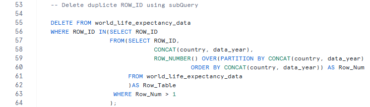
Delete duplicate ROW_ID using subQuery

- Delete duplicate rows from the main table (world_life_expectancy_data).

- A subquery uses ROW_NUMBER() to rank rows within each duplicate group (country + data_year).

- Only rows with Row_Num > 1 are considered duplicates.

- Keeps the first occurrence and removes all extra duplicates.

Cross-check if there are any duplicate rows left

Result:

3.      NULL values in Status column - Identify and Populate them

Identify if there are any NULL values in STATUS column

Result:

Logic:

• Identify distinct values in the status column.

• Map each country to its existing non-NULL status values.

• For any country with NULL in status, fill in the value using the corresponding non-NULL entry for that country.

Check for DISTINCT entries in STATUS column

Result:

Check countries with 'Developing' status

Result:

Check countries with 'Developed' status

Result:

Update NULL entries in STATUS column for 'Developing' countries

- Updates rows in world_life_expectancy_data where STATUS is currently NULL.

- Uses a correlated subquery with EXISTS to check:

• If the same country already has at least one row marked as 'Developing'.

• Ensures that status in the subquery is not NULL.

- If such a row exists, the NULL status is updated to 'Developing'.

- Effectively fills missing STATUS values for countries known to be 'Developing'.

Result:

Update NULL entries in STATUS column for 'Developed' countries

- Updates rows in world_life_expectancy_data where STATUS is currently NULL.

- Uses a correlated subquery with EXISTS to check:

    • If the same country already has at least one row marked as 'Developed'.

    • Ensures that status in the subquery is not NULL.

- If such a row exists, the NULL status is updated to 'Developed'.

- Effectively fills missing STATUS values for countries known to be 'Developed'.

Result:

Cross-check if any NULL values left in STATUS column

Result:

4.      NULL values in Life_Expectancy column - Identify and Populate them

Identify if there are any NULL values in LIFE_EXPECTANCY column

Result:

Logic:

• Identify the rows where life_expectancy is missing.

• For each missing value, locate the previous and next year’s life_expectancy for the same country.

• Calculate the average of the previous and next year’s values.

• Fill the missing life_expectancy with the calculated average.

Update missing life_expectancy values by average of adjacent years

- Self-join the table:

    • t2 = previous year record

    • t3 = next year record

- Match rows based on country and year differences:

    • t2.data_year = t3.data_year - 2 (ensures a one-year gap on both sides)

    • t1.data_year = t2.data_year + 1 (target year sits between prev & next)

- Update only rows where 'life_expectancy' is NULL.

- Use ROUND(..., 1) to keep a single decimal place.

Result:

Cross-check if any NULL values left in LIFE_EXPECTANCY column

Result:

Comparing NULL entries in life_expectancy after filling them with the average of adjacent years.

Before:

After:

Step 3: EDA - Exploratory Data Analysis (using SQL in Snowflake)

Now that the data is cleaned, we can proceed with Exploratory Data Analysis (EDA) to understand patterns, detect anomalies, test hypotheses, and summarize key insights.

1.      Find which countries improved life expectancy the most over time.

- For each country:

    • Take the minimum life expectancy (earliest year available)

    • Take the maximum life expectancy (latest year available)

    • Calculate the improvement as (MAX - MIN), rounded to 1 decimal place

- Exclude countries where life expectancy values are 0

- Finally, order countries by the biggest improvement (highest gains first)

Result:

Conclusion:

Developing countries such as Haiti, Zimbabwe, and Eritrea, which once had life expectancy below 50 years, showed significant progress over the past 15 years. For example, Haiti recorded the largest gain, with life expectancy rising by 28 years. In contrast, developed countries exhibited minimal improvement, as their life expectancy was already high and drastic changes were unlikely.

2.      Calculate the average life expectancy across all countries for each year

- For each year (data_year):

    • Compute the average life expectancy, rounded to 2 decimal places.

    • Exclude years where any country has life expectancy = 0 (to avoid invalid or missing data).

- Order the results chronologically by year.

Result:

Conclusion:

The global average life expectancy increased steadily from 66.75 years in 2007 to 71.62 years in 2022, reflecting a consistent upward trajectory over 15 years.

3.      Analyze the relationship between life expectancy and GDP

- For each country:

    • Calculate the average life expectancy across all available years (rounded to 1 decimal place).

    • Calculate the average GDP across all available years (rounded to 1 decimal place).

    • Exclude countries where either value is 0 (invalid data).

- Order the results by average GDP in descending order, so the wealthiest countries (highest GDP) appear first.

Result:

- Order the results by average GDP in ascending order, so the least wealthy countries (lowest GDP) appear first.

Result:

Compare life expectancy between high-GDP and low-GDP groups

- Classification:

• High GDP: GDP >= 1500

• Low GDP: GDP <= 1500

- For each group:

   • Count how many records (rows) fall into the group.

   • Calculate the average life expectancy for that group.

- The result shows overall counts and average life expectancy

- for high-GDP vs low-GDP countries, enabling a direct comparison.

Result:

Conclusion:

The analysis revealed a strong positive correlation between GDP and life expectancy. Countries with higher GDP generally enjoy longer life expectancy, while low-GDP countries lag behind.

4.      Analyze average health, financial and social indicators based on country status

Analyze average health indicators based on country status

Result:

Conclusion:

There is a clear disparity in health indicators between developed and developing countries, with developed nations benefitting from better healthcare infrastructure. Interestingly, polio prevalence was found to be higher in developed countries, largely due to aggressive eradication campaigns undertaken by developing nations over the past two decades.

Compare social and financial metrics across country statuses

Result:

Conclusion:

Developed countries consistently outperform developing countries in social and financial indicators, reflecting broader access to resources, education, and economic opportunities.

5.      Analyze average health, financial and social indicators based on country status

Result:

Conclusion:

Developed countries (79.2 yrs) live longer than developing ones (66.8 yrs).

6.      Rolling Adult Mortality Rate

Result:

Conclusion:

In the UK Life expectancy gradually increased, while adult mortality showed a steady decline over 15 years.

Limitations of the data:

This dataset does not include population figures, so mortality values cannot be normalized or compared against population size. At this stage, we can contact stakeholders and ask for more data (e.g., population, socioeconomic factors, healthcare access) to enable a more robust exploratory data analysis (EDA).

(Note: These queries represent sample EDA exercises created for portfolio purposes. The dataset allows for many more analyses, such as regional comparisons, trend forecasting, and correlations with socioeconomic indicators.)

This curated data can now be used for advanced visualization in Power BI or Tableau by connecting these tools directly to Snowflake through their built-in connectors.

Conclusion:

The ELT project demonstrates how a structured pipeline can convert raw, inconsistent data into a clean, analytics-ready dataset. The final solution highlights my ability to manage the full data workflow — from automated ingestion to SQL-based transformation and insightful analysis. This project reflects my capability to deliver scalable, cloud-based data solutions that turn messy input into actionable insights.

Lessons Learned:

• Automating ingestion with Fivetran ensures repeatability and eliminates manual overhead

  
  

• Systematic SQL cleaning (handling duplicates, NULLs, and data alignment) is essential before EDA

  
  

• Using adjacent-year interpolation for missing life expectancy values preserved dataset continuity

  
  

• ELT provides more flexibility than ETL in cloud environments, enabling faster iterations and leveraging compute at scale

  
  

• A structured ELT pipeline makes exploratory and advanced analytics more reliable and scalable

Author:

Mukesh Shirke

mukeshshirke12@gmail.com